Examples
Here’s a basic example to get you started with movingpeople:
“many-one” route creation
from movingpeople import visualise_route, generate_routes
import osmnx as ox

# Search query for a geographic area
query = "City of Westminster"
# Get the walking network for the query location
G = ox.graph.graph_from_place(query, network_type="walk", simplify=True)
# Project the graph to WGS84
Gp = ox.project_graph(G, to_crs="4326")

# To make a single route with a randomised origin and fixed destination and randomised start time between a range.
data = generate_routes(
              Gp,
              time_from="2020-02-26 21:42:53",
              time_strategy="fixed",
              route_strategy="many-one",
              origin_destination_coords=[51.499127, -0.153522],
              total_routes=5,
              walk_speed=1.4,
              frequency="1s",
              )

# Visualise the results in keplerGL
visualise_route(data, 500)
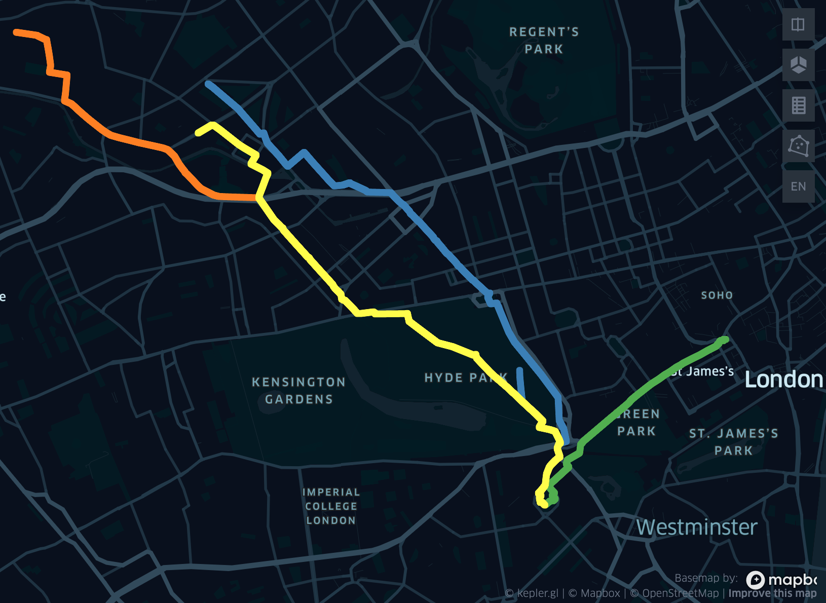
In the example above, we first create a Graph object to define the transportation network. We then generate five routes which have the same start time, randomised origins and a fixed destinations.
Here are the results when visualised using keplerGL:
“many-many” route creation
# To make a single route with a randomised origin and destination and randomised start time between a range.
data = generate_routes(
              Gp,
              time_from="2020-02-26 21:42:53",
              time_until="2020-02-26 22:42:53",
              time_strategy="random",
              route_strategy="many-many",
              origin_destination_coords=None,
              total_routes=12,
              walk_speed=1.4,
              frequency="1s",
              )
   # Visualise the results in keplerGL
   visualise_route(data, 500)
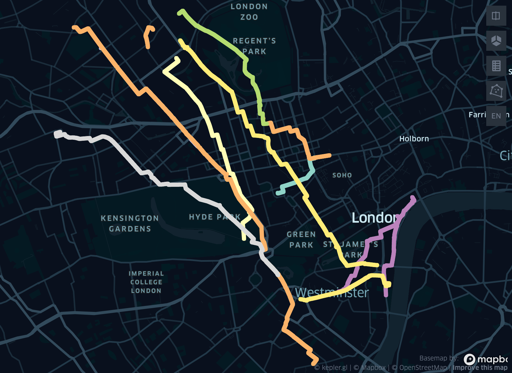
This example makes twelve randomised routes, with each route having a randomised start time between a range.
Here are the results when visualised using keplerGL:
There are many more combinations to experiment with, but to summarise:
Fixed and/or randomised origins
Fixed and/or randomised destinations
n number of routes
Fixed or randomised route start times
Flexible walking speed and point frequency along routes